What is wrong with VAEs?
Latent Variable Models
Suppose you would like to model the world in terms of the probability distribution over its possible states \(p(\mathbf{x})\) with \(\mathbf{x} \in \mathcal{R}^D\). The world may be complicated and we do not know what form \(p(\mathbf{x})\) should have. To account for it, we introduce another variable \(\mathbf{z} \in \mathcal{R}^d\), which describes, or explains the content of \(\mathbf{x}\). If \(\mathbf{x}\) is an image, \(\mathbf{z}\) can contain information about the number, type and appearance of objects visible in the scene as well as the background and lighting conditions. This new variable allows us to express \(p(\mathbf{x})\) as an infinite mixture model,
\[p(\mathbf{x}) = \int p(\mathbf{x} \mid \mathbf{z}) p(\mathbf{z})~d \mathbf{z}. \tag{1}\]It is a mixture model, because for every possible value of \(\mathbf{z}\), we add another conditional distribution to \(p(\mathbf{x})\), weighted by its probability.
Having a setup like that, it is interesting to ask what the latent variables \(\mathbf{z}\) are, given an observation \(\mathbf{x}\). Namely, we would like to know the posterior distribution \(p(\mathbf{z} \mid \mathbf{x})\). However, the relationship between \(\mathbf{z}\) and \(\mathbf{x}\) can be highly non-linear (e.g. implemented by a multi-layer neural network) and both \(D\), the dimensionality of our observations, and \(d\), the dimensionality of the latent variable, can be quite large. Since both marginal and posterior probability distributions require evaluation of the integral in eq. (1), they are intractable.
We could try to approximate eq. (1) by Monte-Carlo sampling as \(p(\mathbf{x}) \approx \frac{1}{M} \sum_{m=1}^M p(\mathbf{x} \mid \mathbf{z}^{(m)})\), \(\mathbf{z}^{(m)} \sim p(\mathbf{z})\), but since the volume of \(\mathbf{z}\)-space is potentially large, we would need millions of samples of \(\mathbf{z}\) to get a reliable estimate.
To train a probabilistic model, we can use a parametric distribution - parametrised by a neural network with parameters \(\theta \in \Theta\). We can now learn the parameters by maximum likelihood estimation,
\[\theta^\star = \arg \max_{\theta \in \Theta} p_\theta(\mathbf{x}). \tag{2}\]The problem is, we cannot maximise an expression (eq. (1)), which we can’t even evaluate. To improve things, we can resort to importance sampling (IS). When we need to evaluate an expectation with respect to the original (nominal) probability density function (pdf), IS allows us to sample from a different probability distribution (proposal) and then weigh those samples with respect to the nominal pdf. Let \(q_\phi ( \mathbf{z} \mid \mathbf{x})\) be our proposal - a probability distribution parametrised by a neural network with parameters \(\phi \in \Phi\). We can write
\[p_\theta(\mathbf{x}) = \int p(\mathbf{z}) p_\theta (\mathbf{x} \mid \mathbf{z})~d \mathbf{z} =\\ \mathbb{E}_{p(\mathbf{z})} \left[ p_\theta (\mathbf{x} \mid \mathbf{z} )\right] = \mathbb{E}_{p(\mathbf{z})} \left[ \frac{q_\phi ( \mathbf{z} \mid \mathbf{x})}{q_\phi ( \mathbf{z} \mid \mathbf{x})} p_\theta (\mathbf{x} \mid \mathbf{z} )\right] = \mathbb{E}_{q_\phi ( \mathbf{z} \mid \mathbf{x})} \left[ \frac{p_\theta (\mathbf{x} \mid \mathbf{z} ) p(\mathbf{z})}{q_\phi ( \mathbf{z} \mid \mathbf{x})} )\right]. \tag{3}\]From importance sampling literature we know that the optimal proposal is proportional to the nominal pdf times the function, whose expectation we are trying to approximate. In our setting, that function is just \(p_\theta (\mathbf{x} \mid \mathbf{z} )\). From Bayes’ theorem, \(p(z \mid x) = \frac{p(x \mid z) p (z)}{p(x)}\), we see that the optimal proposal is proportional to the posterior distribution, which is of course intractable.
Rise of a Variational Autoencoder
Fortunately, it turns out, we can kill two birds with one stone: by trying to approximate the posterior with a learned proposal, we can efficiently approximate the marginal probability \(p_\theta(\mathbf{x})\). A bit by accident, we have just arrived at an autoencoding setup. To learn our model, we need
- \(p_\theta ( \mathbf{x}, \mathbf{z})\) - the generative model, which consists of
- \(p_\theta ( \mathbf{x} \mid \mathbf{z})\) - a probabilistic decoder, and
- \(p ( \mathbf{z})\) - a prior over the latent variables,
- \(q_\phi ( \mathbf{z} \mid \mathbf{x})\) - a probabilistic encoder.
To approximate the posterior, we can use the KL-divergence (think of it as a distance between probability distributions) between the proposal and the posterior itself; and we can minimise it.
\[KL \left( q_\phi (\mathbf{z} \mid \mathbf{x}) || p_\theta(\mathbf{z} \mid \mathbf{x}) \right) = \mathbb{E}_{q_\phi (\mathbf{z} \mid \mathbf{x})} \left[ \log \frac{q_\phi (\mathbf{z} \mid \mathbf{x})}{p_\theta(\mathbf{z} \mid \mathbf{x})} \right] \tag{4}\]Our new problem is, of course, that to evaluate the KL we need to know the posterior distribution. Not all is lost, for doing a little algebra can give us an objective function that is possible to compute.
\[\begin{align} KL &\left( q_\phi (\mathbf{z} \mid \mathbf{x}) || p_\theta(\mathbf{z} \mid \mathbf{x}) \right)\\ &=\mathbb{E}_{q_\phi (\mathbf{z} \mid \mathbf{x})} \left[ \log q_\phi (\mathbf{z} \mid \mathbf{x}) - \log p_\theta(\mathbf{z} \mid \mathbf{x}) \right]\\ &=\mathbb{E}_{q_\phi (\mathbf{z} \mid \mathbf{x})} \left[ \log q_\phi (\mathbf{z} \mid \mathbf{x}) - \log p_\theta(\mathbf{z}, \mathbf{x}) \right] + \log p_\theta(\mathbf{x})\\ &= -\mathcal{L} (\mathbf{x}; \theta, \phi) + \log p_\theta(\mathbf{x}) \tag{5} \end{align}\]Where on the second line I expanded the logarithm, on the third line I used the Bayes’ theorem and the fact that \(p_\theta (\mathbf{x})\) is independent of \(\mathbf{z}\). \(\mathcal{L} (\mathbf{x}; \theta, \phi)\) in the last line is a lower bound on the log probability of data \(p_\theta (\mathbf{x})\) - the so-called evidence-lower bound (ELBO). We can rewrite it as
\[\log p_\theta(\mathbf{x}) = \mathcal{L} (\mathbf{x}; \theta, \phi) + KL \left( q_\phi (\mathbf{z} \mid \mathbf{x}) || p_\theta(\mathbf{z} \mid \mathbf{x}) \right), \tag{6}\] \[\mathcal{L} (\mathbf{x}; \theta, \phi) = \mathbb{E}_{q_\phi (\mathbf{z} \mid \mathbf{x})} \left[ \log \frac{ p_\theta (\mathbf{x}, \mathbf{z}) }{ q_\phi (\mathbf{z} \mid \mathbf{x}) } \right]. \tag{7}\]We can approximate it using a single sample from the proposal distribution as
\[\mathcal{L} (\mathbf{x}; \theta, \phi) \approx \log \frac{ p_\theta (\mathbf{x}, \mathbf{z}) }{ q_\phi (\mathbf{z} \mid \mathbf{x}) }, \qquad \mathbf{z} \sim q_\phi (\mathbf{z} \mid \mathbf{x}). \tag{8}\]We train the model by finding \(\phi\) and \(\theta\) (usually by stochastic gradient descent) that maximise the ELBO:
\[\phi^\star,~\theta^\star = \arg \max_{\phi \in \Phi,~\theta \in \Theta} \mathcal{L} (\mathbf{x}; \theta, \phi). \tag{9}\]By maximising the ELBO, we (1) maximise the marginal probability or (2) minimise the KL-divergence, or both. It is worth noting that the approximation of ELBO has the form of the log of importance-sampled expectation of \(f(\mathbf{x}) = 1\), with importance weights \(w(\mathbf{x}) = \frac{ p_\theta (\mathbf{x}, \mathbf{z}) }{ q_\phi (\mathbf{z} \mid \mathbf{x})}\).
What is wrong with this estimate?
If you look long enough at importance sampling, it becomes apparent that the support of the proposal distribution should be wider than that of the nominal pdf - both to avoid infinite variance of the estimator and numerical instabilities. In this case, it would be better to optimise the reverse \(KL(p \mid\mid q)\), which has mode-averaging behaviour, as opposed to \(KL(q \mid\mid p)\), which tries to match the mode of \(q\) to one of the modes of \(p\). This would typically require taking samples from the true posterior, which is hard. Instead, we can use IS estimate of the ELBO, introduced as Importance Weighted Autoencoder (IWAE). The idea is simple: we take \(K\) samples from the proposal and we use an average of probability ratios evaluated at those samples. We call each of the samples a particle.
\[\mathcal{L}_K (\mathbf{x}; \theta, \phi) \approx \log \frac{1}{K} \sum_{k=1}^{K} \frac{ p_\theta (\mathbf{x},~\mathbf{z^{(k)}}) }{ q_\phi (\mathbf{z^{(k)}} \mid \mathbf{x}) }, \qquad \mathbf{z}^{(k)} \sim q_\phi (\mathbf{z} \mid \mathbf{x}). \tag{10}\]This estimator has been shown to optimise the modified KL-divergence \(KL(q^{IS} \mid \mid p^{IS})\), with \(q^{IS}\) and \(p^{IS}\) defined as \(q^{IS} = q^{IS}_\phi (\mathbf{z} \mid \mathbf{x}) = \frac{1}{K} \prod_{k=1}^K q_\phi ( \mathbf{z}^{(k)} \mid \mathbf{x} ), \tag{11}\)
\[p^{IS} = p^{IS}_\theta (\mathbf{z} \mid \mathbf{x}) = \frac{1}{K} \sum_{k=1}^K \frac{ q^{IS}_\phi (\mathbf{z} \mid \mathbf{x}) }{ q_\phi (\mathbf{z^{(k)}} \mid \mathbf{x}) } p_\theta (\mathbf{z}^{(k)} \mid \mathbf{x}). \tag{12}\]While similar to the original distributions, \(q^{IS}\) and \(p^{IS}\) allow small variations in \(q\) and \(p\) that we would not have expected. Optimising this lower bound leads to better generative models, as shown in the original paper. It also leads to higher-entropy (wider, more scattered) estimates of the approximate posterior \(q\), effectively breaking the mode-matching behaviour of the original KL-divergence. As a curious consequence, if we increase the number of particles \(K\) to infinity, we no longer need the inference model \(q\).
What is wrong with IWAE?
The importance-weighted ELBO, or the IWAE, generalises the original ELBO: for \(K=1\), we have \(\mathcal{L}_K = \mathcal{L}_1 = \mathcal{L}\). It is also true that \(\log p(\mathbf{x}) \geq \mathcal{L}_{n+1} \geq \mathcal{L}_n \geq \mathcal{L}_1\). In other words, the more particles we use to estimate \(\mathcal{L}_K\), the closer it gets in value to the true log probability of data - we say that the bound becomes tighter. This means that the gradient estimator, derived by differentiating the IWAE, points us in a better direction than the gradient of the original ELBO would. Additionally, as we increase \(K\), the variance of that gradient estimator shrinks.
It is great for the generative model, but, as we shown in our recent paper Tighter Variational Bounds are Not Necessarily Better, it turns out to be problematic for the proposal. The magnitude of the gradient with respect to proposal parameters goes to zero with increasing \(K\), and it does so much faster than its variance.
Let \(\Delta (\phi)\) be a minibatch estimate of the gradient of an objective function we’re optimising (e.g. ELBO) with respect to \(\phi\). If we define signal-to-noise ratio (SNR) of the parameter update as
\[SNR(\phi) = \frac{ \left| \mathbb{E} \left[ \Delta (\phi ) \right] \right| }{ \mathbb{V} \left[ \Delta (\phi ) \right]^{\frac{1}{2}} }, \tag{13}\]where \(\mathbb{E}\) and \(\mathbb{V}\) are expectation and variance, respectively, it turns out that SNR increases with \(K\) for \(p_\theta\), but it decreases for \(q_\phi\). The conclusion here is simple: the more particles we use, the worse the inference model becomes. If we care about representation learning, we have a problem.
Better estimators
We can do better than the IWAE, as we’ve shown in our paper. The idea is to use separate objectives for the inference and the generative models. By doing so, we can ensure that both get non-zero low-variance gradients, which lead to better models.
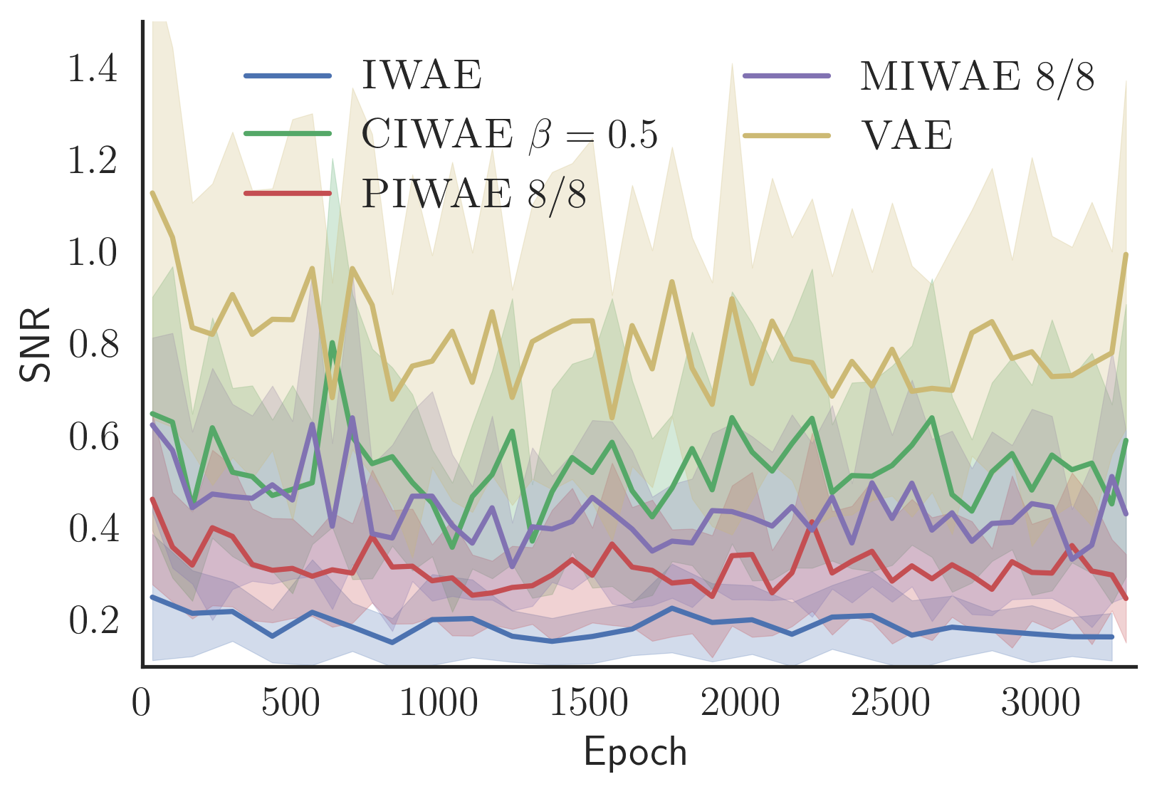
In the above plot, we compare SNR of the updates of parameters \(\phi\) of the proposal \(q_\phi\) acorss training epochs. VAE, which shows the highest SNR, is trained by optimising \(\mathcal{L}_1\). IWAE, trained with \(\mathcal{L}_{64}\), has the lowest SNR. The three curves in between use different combinations of \(\mathcal{L}_{64}\) for the generative model and \(\mathcal{L}_8\) or \(\mathcal{L}_1\) for the inference model. While not as good as the VAE under this metric, they all lead to training better proposals and generative models than either VAE or IWAE.
As a, perhaps surprising, side effect, models trained with our new estimators achieve higher \(\mathcal{L}_{64}\) bounds than the IWAE itself trained with this objective. Why? By looking at the effective sample-size (ESS) and the marginal log probability of data, it looks like optimising \(\mathcal{L}_1\) leads to producing the best quality proposals, but the worst generative models. If we combine a good proposal with an objective that leads to good generative models, we should be able to provide lower-variance estimate of this objective and thus learn even better models. Please see our paper for details.
Further Reading
- More flexible proposals: Normalizing Flows tutorial by Eric Jang part 1 and part 2
- More flexible likelihood function: A post on Pixel CNN by Sergei Turukin
- Extension of IWAE to sequences: Chris Maddison et. al., “FIVO” and Tuan Anh Le et. al., “AESMC”
Acknowledgements
I would like to thank Neil Dhir and Anton Troynikov for proofreading this post and suggestions on how to make it better.