Objects play a central role in computer vision and, increasingly, machine learning research. With many applications depending on object detection in images and videos, the demand for accurate and efficient algorithms is high. More generally, knowing about objects is essential for understanding and interacting with our environments. Usually, object detection is posed as a supervised learning problem, and modern approaches typically involve training a CNN to predict the likelihood of whether an object exists at a given image location (and maybe the corresponding class), see e.g. here.

While modern methods can achieve human-like performance in object recognition, they need to consume staggering amounts of data to do so. This is in stark contrast to mammals, who learn to recognize and localize objects with no supervision. It is difficult to say what exactly makes mammals so good at learning, but we can imagine that self-supervision¹ and inductive biases present in their sophisticated computing hardware (or rather ‘wetware’; that is brains) both play a huge role. These intuitions have led us to develop an unsupervised version of capsule networks, see Figure 1 for an overview, whose inductive biases give rise to object-centric latent representations, which are learned in a self-supervised way—simply by reconstructing input images. Clustering learned representations was enough to allow us to achieve unsupervised state-of-the-art classification performance on MNIST (98.5%) and SVHN (55%). In the remainder of this blog, I will try to explain what those inductive biases are, how they are implemented and what kind of things are possible with this new capsule architecture. I will also try to explain how this new version differs from previous versions of capsule networks.

Why do we care about equivariances?

I think it is fair to say that deep learning would not be so popular if not for CNNs and the 2012 AlexNet paper. CNNs learn faster than non-convolutional image models due to (1) local connectivity and (2) parameter sharing across spatial locations. The former restricts what can be learned, but is sufficient to learn correlations between nearby pixels, which turns out to be important for images. The latter makes learning easier since parameter updates benefit from more signal. It also results in translation equivariance, which means that, when the input to a CNN is shifted, the output is shifted by an equal amount, while remaining unchanged otherwise. Formally, a function \(f(\mathbf{x})\) is equivariant to any transformation \(T \in \mathcal{T}\) if \(\forall_{T \in \mathcal{T}} Tf(\mathbf{x}) = f(T\mathbf{x})\). That is, applying any transformation to the input of the function has the same effect as applying that transformation to the output of the function. Invariance is a related notion, and the function \(f\) is invariant if \(\forall_{T \in \mathcal{T}} f(\mathbf{x}) = f(T\mathbf{x})\)—applying transformations to the input does not change the output.

Being equivariant helps with learning and generalization—for example, a model does not have to see the object placed at every possible spatial location in order to learn how to classify it. For this reason, it would be great to have neural nets that are equivariant to other affine degrees of freedom like rotation, scale, and shear, but this is not very easy to achieve, see e.g. group equivariant conv nets.

Equivariance to different transformations can be learned approximately, but it requires vast data augmentation and a considerably higher training cost. Augmenting data with random crops or shifts helps even with training translation-equivariant CNNs since these are typically followed by fully-connected layers, which have to learn to handle different positions. Other affine transformations² are not easy to augment with, as they would require access to full three-dimensional scene models. Even if scene models were available, we would need to augment data with combinations of different transformations, which would result in an absolutely enormous dataset. The problem is exacerbated by the fact that objects are often composed of parts, and it would be best to capture all possible configurations of object parts. Spatial Transformer Networks and this followup work provide one way of learning affine equivariances but do not address the fact that objects can undergo local transformations.

Capsules learn equivariant object representations

Instead of building models that are globally equivariant to affine transformations, we can rely on the fact that scenes often contain many complicated objects, which in turn are composed of simpler parts. By definition, parts exhibit less variety in their appearance and shape than full objects, and consequently, they should be easier to learn from raw pixels. Objects can then be recognized from parts and their poses, given that we can learn how parts come together to form different objects, as in Figure 2. The caveat here is that we still need to learn a part detector, and it needs to predict part poses (i.e. translation, rotation, and scale) too. We hypothesize that this should be much simpler than learning an end-to-end object detector with similar capabilities.

Since poses of any entities present in a scene change with the location of an observer (or rather the chosen coordinate system), then a detector that can correctly identify poses of parts produces a viewpoint-equivariant part representation. Since object-part relationships do not depend on the particular vantage point, they are viewpoint-invariant. These two properties, taken together, result in viewpoint-equivariant object representations.

The issue with the above is that the corresponding inference process, that is, using previously discovered parts to infer objects, is difficult since every part can belong to at most one object. Previous versions of capsules solved this by iteratively refining the assignment of parts to objects (also known as routing). This proved to be inefficient in terms of both computation and memory and made it impossible to scale to bigger images. See e.g. here for an overview of previous capsule networks.

Can an arbitrary neural net learn capsule-like representations?

Original capsules are a type of a feed-forward neural network with a specific structure and are trained for classification. Incidentally, we know that classification corresponds to inference, which is the inverse process of generation, and as such is more difficult. To see this, think about Bayes’ rule: this is why posterior distributions are often much more complicated than the prior or likelihood terms³.

Instead, we can use the principles introduced by capsules to build a generative model (decoder) and a corresponding inference network (encoder). Generation is simpler, since we can have any object generate arbitrarily many parts, and we do not have to deal with constraints encountered in inference. Complicated inference can then be left to your favorite neural network, which is going to learn appropriate latent representations. Since the decoder uses capsules machinery, it is viewpoint equivariant by design. It follows that the encoder has to learn representations that are also viewpoint equivariant, at least approximately.

A potential disadvantage is that, even though the latent code might be viewpoint equivariant, in the sense that it explicitly encodes object coordinates, the encoder itself need not be viewpoint equivariant. This means that, if the model sees an object from a very different point of view than it is used to, it may fail to recognize the object. Interestingly, this seems to be in line with human perception, as noted recently by Geoff Hinton in his Turing Award lecture, where he uses a thought experiment to illustrate this. If you are interested, you can watch the below video for about 2.5 minutes.

Here is a simplified version of the example in the video, see Figure 3: imagine a square, and tilt it by 45 degrees, look away, and look at it again. Can you see a square? Or does the shape resemble a diamond? Humans tend to impose coordinate frames on the objects they see, and the coordinate frame is one of the features that let us recognize the objects. If the coordinate frame is very different from the usual one, we may have problems recognizing the correct shape.

Why bother?

I hope I have managed to convince you that learning capsule-like representations is possible. Why is it a good idea? While we still have to scale the method to complicated real-world imagery, the initial results are quite promising. It turns out that the object capsules can learn to specialize to different types of objects. When we clustered the presence probabilities of object capsules we found that, to our surprise, representations of objects from the same class are grouped tightly together. Simply looking up the label that examples in a given cluster correspond to resulted in state-of-the-art unsupervised classification accuracy on two datasets: MNIST (98.5%) and SVHN (55%). We also took a model trained on MNIST and simulated unseen viewpoints by performing affine transformations of the digits, and also achieved state-of-the-art unsupervised performance (92.2%), which shows that learned representations are in fact robust to viewpoint changes. Results on Cifar10 are not quite as good, but still promising. In future work, we are going to explore more expressive approaches to image reconstruction, instead of using fixed templates, and hopefully, scale up to more complicated data.

Technical bits

This is the end of high-level intuitions, and we now proceed to some technical descriptions, albeit also high-level ones. This might be a good place to stop reading if you are not into that sort of thing.

In the following, I am going to describe the decoding stack of our model, and you can think of it as a (deterministic) generative model. Next, I will describe an inference network, which provides the capsule-like representations.

How can we turn object prototypes into an image?

Let us start by defining what a capsule is.

We define a capsule as a specialized part of a model that describes an abstract entity, e.g. a part or an object. In the following, we will have object capsules, which recognize objects from parts, and part capsules, which extract parts and poses from an input image. Let capsule activation be a group of variables output by a single capsule. To describe an object, we would like to know (1) whether it exists, (2) what it looks like and (3) where it is located⁴. Therefore, for an object capsule \(k\), its activations consist of (1) a presence probability \(a_k\), (2) a feature vector \(\mathbf{c_k}\), and (3) a \(3\times 3\) pose matrix \(OV_k\), which represents the geometrical relationship between the object and the viewer (or some central coordinate system). Similar features can be used to describe parts, but we will simplify the setup slightly and assume that parts have a fixed appearance and only their pose can vary. Therefore, for the \(m^\mathrm{th}\) part capsule, its activations consist of the probability \(d_m\) that the part exists, and a \(6\)-dimensional⁵ pose \(\mathbf{x}_m\), which represents the position and orientation of the given part in the image. As indicated by notation, there are several object capsules and potentially many part capsules.

Since every object can have several parts, we need a mechanism to turn an object capsule activation into several part capsule activations. To this end, for every object capsule, we learn a set of \(3\times 3\) transformation matrices \(OP_{k,m}\), representing the geometrical relationship between an object and its parts. These matrices are encouraged to be constant, although we do allow a weak dependence on the object features \(\mathbf{c}_k\) to account for small deformations. Since any part can belong to only one object, we gather predictions from all object capsules corresponding to the same part capsule and arrange them into a mixture. If the model is confident that a particular object should be responsible for a given part, then this will be reflected in the mixing probabilities of the mixture. In this case, sampling from the mixture will be similar to just taking argmax over the mixing proportions while also accounting for uncertainty in the assignment. Finally, we explain parts by independent Gaussian mixtures; this is a simplifying assumption saying that a choice of a parent for one part should not influence the choice of parents for other parts.

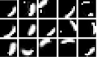
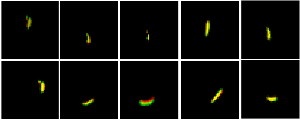
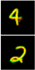
Having generated part poses, we can take parts, apply affine transformations parametrized by the corresponding poses as in Spatial Transformer, and assemble the transformed parts into an image (Figure 4). But wait—we need to get the parts first! Since we assumed that parts have fixed appearance, we are going to learn a bank of fixed parts by gradient descent. Each part is like an image, just smaller, and can be seen as a “template”. To give an example, a good template for MNIST digits would be a stroke, like in the famous paper from Lake et. al. or the left-hand side of Figure 4.

Where do we get capsule parameters from?

Above, we define a generative process that can transform object and part capsule activations into images. But to obtain capsule activations describing a particular image, we need to run some sort of inference. In this case, we will just use neural networks to amortize inference, like in a VAE, (see this post for more details on VAEs). In other words, neural nets will predict capsule activations directly from the image. We will do this in two stages. Firstly, given the image, we will have a neural net predict pose parameters and presence probabilities for every part from our learnable bank of parts. Secondly, a separate neural net will look at the part parameters and will try to directly predict object capsule activations. These two stages correspond to two stages of the generative process we outlined; we can now pair each of the stages with the corresponding generative stage and arrive at two autoencoders. The first one, Part Capsule Autoencoder (PCAE), detects parts and recombines them into an image. The second one, Object Capsule Autoencoder (OCAE), organizes parts into objects. Below, we describe their architecture and some of our design choices.

Inferring parts and poses

The PCAE uses a CNN-based encoder, but with tweaks. Firstly, notice that for \(M\) parts, we need \(M \times (6 + 1)\) predicted parameters. That is, for every part we need \(6\) parameters of an affine transformation \(\mathbf{x}_m\) (we work in two dimensions) and a probability \(d_m\) of the part being present; we could also predict some additional parameters; in fact we do, but we omit the details here for clarity—see the paper for details. It turns out that using a fully-connected layer after a CNN does not work well here; see the paper for details. Instead, we project the outputs of the CNN to \(M \times (6 + 1 + 1)\) feature maps using \(1\times 1\) convolutions, where we added an extra feature map for each part capsule. This extra feature map will serve as an attention mask: we normalize it spatially via a softmax, multiply with the remaining 7 feature maps, and sum each dimension independently across spatial locations. This is similar to global-average pooling, but allows the model to focus on a specific location; we call it attention-based pooling.

We can then use part presence probabilities and part poses to select and affine-transform learned parts, and assemble them into an image. Every transformed part is treated as a spatial Gaussian mixture component, and we train PCAE by maximizing the log-likelihood under this mixture.

Organizing parts into objects

Knowing what parts there are in an image and where they are might be useful, but in the end, we care about the objects that they belong to. Previous capsules used an EM-based inference procedure to make parts vote for objects. This way, each part could start by initially disagreeing and voting on different objects, but eventually, the votes would converge to a set of only a few objects. We can also see inference as compression, where a potentially large set of parts is explained by a potentially very sparse set of objects. Therefore, we try to predict object capsule activations directly from the poses and presence probabilities of parts. The EM-based inference tried to cluster part votes around objects. We follow this intuition and use the Set Transformer with \(K\) outputs to encode part activations. Set Transformer has been shown to work well for amortized-clustering-type problems, and it is permutation invariant. Part capsule activations describe parts, not pixels, which can have arbitrary positions in the image, and in that sense have no order. Therefore, set-input neural networks seem to be a better choice than MLPs—a hypothesis corroborated by an ablation study we have in the paper.

Each output of the Set Transformer is fed into a separate MLP, which then outputs all activations for the corresponding object capsule. We also use a number of sparsity losses applied to the object presence probabilities; these are necessary to make object capsules specialize to different types of objects, please see the paper for details. The OCAE is trained by maximizing the likelihood of part capsule activations under a Gaussian mixture of predictions from object capsules, subject to sparsity constraints.

Summary

In summary, a Stacked Capsule Autoencoder is composed of:

• the PCAE encoder: a CNN with attention-based pooling,
• the OCAE encoder: a Set Transformer,
• the OCAE decoder:
  • \(K\) MLPs, one for every object capsule, which predicts capsule parameters from Set Transformer’s outputs,
  • \(K \times M\) constant \(3 \times 3\) matrices representing constant object-part relationships,
• and the PCAE decoder, which is just \(M\) constant part templates, one for each part capsule.

SCAE defines a new method for representation learning, where an arbitrary encoder learns viewpoint-equivariant representations by inferring parts and their poses and groups them into objects. This post provides motivation as well as high-level intuitions behind this idea, and an overview of the method. The major drawback of the method, as of now, is that the part decoder uses fixed templates, which are insufficient to model complicated real-world images. This is also an exciting avenue for future work, together with deeper hierarchies of capsules and extending capsule decoders to three-dimensional geometry. If you are interested in the details, I would encourage you to read the original paper: A. R. Kosiorek, S. Sabour, Y.W. Teh and G. E. Hinton, “Stacked Capsule Autoencoders”, arXiv 2019.

Further reading:

• a series of blog posts explaining previous capsule networks
• the original capsule net paper and the version with EM routing
• a recent CVPR tutorial on capsules and slides by Sara Sabour

Footnotes

Acknowledgements

This work was done during my internship at Google Brain in Toronto in Geoff Hinton’s team. I would like to thank my collaborators: Sara Sabour, Yee Whye Teh and Geoff Hinton. I also thank Ali Eslami and Danijar Hafner for helpful discussions. Big thanks goes to Sandy H. Huang who helped with making figures and editing the paper. Sandy, Adam Goliński and Martin Engelcke provided extensive feedback on this post.