Normalizing Flows
Machine learning is all about probability. To train a model, we typically tune its parameters to maximise the probability of the training dataset under the model. To do so, we have to assume some probability distribution as the output of our model. The two distributions most commonly used are Categorical for classification and Gaussian for regression. The latter case can be problematic, as the true probability density function (pdf) of real data is often far from Gaussian. If we use the Gaussian as likelihood for image-generation models, we end up with blurry reconstructions. We can circumvent this issue by adversarial training, which is an example of likelihood-free inference, but this approach has its own issues.
Gaussians are also used, and often prove too simple, as the pdf for latent variables in Variational Autoencoders (VAEs), which I describe in my previous post. Fortunately, we can often take a simple probability distribution, take a sample from it and then transform the sample. This is equivalent to change of variables in probability distributions and, if the transformation meets some mild conditions, can result in a very complex pdf of the transformed variable. Danilo Rezende formalised this in his paper on Normalizing Flows (NF), which I describe below. NFs are usually used to parametrise the approximate posterior \(q\) in VAEs but can also be applied for the likelihood function.
Change of Variables in Probability Distributions
We can transform a probability distribution using an invertible mapping (i.e. bijection). Let \(\mathbf{z} \in \mathbb{R}^d\) be a random variable and \(f: \mathbb{R}^d \mapsto \mathbb{R}^d\) an invertible smooth mapping. We can use \(f\) to transform \(\mathbf{z} \sim q(\mathbf{z})\). The resulting random variable \(\mathbf{y} = f(\mathbf{z})\) has the following probability distribution:
\[q_y(\mathbf{y}) = q(\mathbf{z}) \left| \mathrm{det} \frac{ \partial f^{-1} }{ \partial \mathbf{z}\ } \right| = q(\mathbf{z}) \left| \mathrm{det} \frac{ \partial f }{ \partial \mathbf{z}\ } \right| ^{-1}. \tag{1}\]We can apply a series of mappings \(f_k\), \(k \in {1, \dots, K}\), with \(K \in \mathbb{N}_+\) and obtain a normalizing flow, first introduced in Variational Inference with Normalizing Flows,
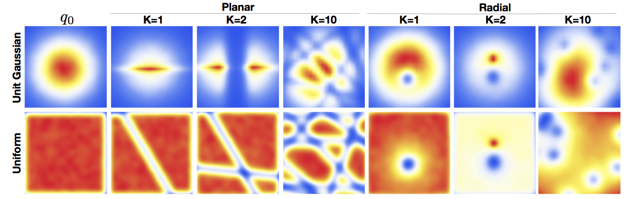
\[\mathbf{z}_K = f_K \circ \dots \circ f_1 (\mathbf{z}_0), \quad \mathbf{z}_0 \sim q_0(\mathbf{z}_0), \tag{2}\] \[\mathbf{z}_K \sim q_K(\mathbf{z}_K) = q_0(\mathbf{z}_0) \prod_{k=1}^K \left| \mathrm{det} \frac{ \partial f_k }{ \partial \mathbf{z}_{k-1}\ } \right| ^{-1}. \tag{3}\]This series of transformations can transform a simple probability distribution (e.g. Gaussian) into a complicated multi-modal one. To be of practical use, however, we can consider only transformations whose determinants of Jacobians are easy to compute. The original paper considered two simple family of transformations, named planar and radial flows.
Simple Flows
Planar Flow
\(f(\mathbf{z}) = \mathbf{z} + \mathbf{u} h(\mathbf{w}^T \mathbf{z} + b), \tag{4}\)
with \(\mathbf{u}, \mathbf{w} \in \mathbb{R}^d\) and \(b \in \mathbb{R}\) and \(h\) an element-wise non-linearity. Let \(\psi (\mathbf{z}) = h' (\mathbf{w}^T \mathbf{z} + b) \mathbf{w}\). The determinant can be easily computed as
\[\left| \mathrm{det} \frac{\partial f}{\partial \mathbf{z}} \right| = \left| 1 + \mathbf{u}^T \psi( \mathbf{z} ) \right|. \tag{5}\]We can think of it as slicing the \(\mathbf{z}\)-space with straight lines (or hyperplanes), where each line contracts or expands the space around it, see figure 1.
Radial Flow
\[f(\mathbf{z}) = \mathbf{z} + \beta h(\alpha, r)(\mathbf{z} - \mathbf{z}_0), \tag{6}\]with \(r = \Vert\mathbf{z} - \mathbf{z}_0\Vert_2\), \(h(\alpha, r) = \frac{1}{\alpha + r}\) and parameters \(\mathbf{z}_0 \in \mathbb{R}^d, \alpha \in \mathbb{R}_+\) and \(\beta \in \mathbb{R}\).
Similarly to planar flows, radial flows introduce spheres in the \(\mathbf{z}\)-space, which either contract or expand the space inside the sphere, see figure 1.
Discussion
These simple flows are useful only for low dimensional spaces, since each transformation affects only a small volume in the original space. As the volume of the space grows exponentially with the number of dimensions \(d\), we need a lot of layers in a high-dimensional space.
Another way to understand the need for many layers is to look at the form of the mappings. Each mapping behaves as a hidden layer of a neural network with one hidden unit and a skip connection. Since a single hidden unit is not very expressive, we need a lot of transformations. Recently introduced Sylvester Normalising Flows overcome the single-hidden-unit issue of these simple flows; for more details please read the paper.
Simple flows are useful for sampling, e.g. as parametrisation of \(q(\mathbf{z})\) in VAEs, but it is very difficult to evaluate probability of a data point that was not sampled from it. This is because the functions \(h\) in planar and radial flow are invertible only in some regions of the \(\mathbf{z}\)-space, and the functional form of their inverse is generally unknown. Please drop a comment if you have an idea how to fix that.
Autoregressive Flows
Enhancing expressivity of normalising flows is not easy, since we are constrained by functions, whose Jacobians are easy to compute. It turns out, though, that we can introduce dependencies between different dimensions of the latent variable, and still end up with a tractable Jacobian. Namely, if after a transformation, the dimension \(i\) of the resulting variable depends only on dimensions \(1:i\) of the input variable, then the Jacobian of this transformation is triangular. As we know, a determinant of a triangular matrix is equal to the product of the terms on the diagonal. More formally, let \(J \in \mathcal{R}^{d \times d}\) be the Jacobian of the mapping \(f\), then
\[y_i = f(\mathbf{z}_{1:i}), \qquad J = \frac{\partial \mathbf{y}}{\partial \mathbf{z}}, \tag{7}\] \[\det{J} = \prod_{i=1}^d J_{ii}. \tag{8}\]I would like to draw your attention to three interesting flows that use the above observation, albeit in different ways, and arrive at mappings with very different properties.
Real Non-Volume Preserving Flows (R-NVP)
R-NVPs are arguably the least expressive but the most generally applicable of the three. Let \(1 < k < d\), \(\circ\) element-wise multiplication and \(\mu\) and \(\sigma\) two mappings \(\mathcal{R}^k \mapsto \mathcal{R}^{d-k}\) (Note that \(\sigma\) is not the sigmoid function). R-NVPs are defined as:
\[\mathbf{y}_{1:k} = \mathbf{z}_{1:k},\\ \mathbf{y}_{k+1:d} = \mathbf{z}_{k+1:d} \circ \sigma(\mathbf{z}_{1:k}) + \mu(\mathbf{z}_{1:k}). \tag{9}\]It is an autoregressive transformation, although not as general as equation (7) allows. It copies the first \(k\) dimensions, while shifting and scaling all the remaining ones. The first part of the Jacobian (up to dimension \(k\)) is just an identity matrix, while the second part is lower-triangular with \(\sigma(\mathbf{z}_{1:k})\) on the diagonal. Hence, the determinant of the Jacobian is
\[\frac{\partial \mathbf{y}}{\partial \mathbf{z}} = \prod_{i=1}^{d-k} \sigma_i(\mathbf{z}_{1:k}). \tag{10}\]R-NVPs are particularly attractive, because both sampling and evaluating probability of some external sample are very efficient. Computational complexity of both operations is, in fact, exactly the same. This allows to use R-NVPs as a parametrisation of an approximate posterior \(q\) in VAEs, but also as the output likelihood (in VAEs or general regression models). To see this, first note that we can compute all elements of \(\mu\) and \(\sigma\) in parallel, since all inputs (\(\mathbf{z}\)) are available. We can therefore compute \(\mathbf{y}\) in a single forward pass. Next, note that the inverse transformation has the following form, with all divisions done element-wise,
\[\mathbf{z}_{1:k} = \mathbf{y}_{1:k},\\ \mathbf{z}_{k+1:d} = (\mathbf{y}_{k+1:d} - \mu(\mathbf{y}_{1:k}))~/~\sigma(\mathbf{y}_{1:k}). \tag{11}\]Note that \(\mu\) and \(\sigma\) are usually implemented as neural networks, which are generally not invertible. Thanks to equation (11), however, they do not have to be invertible for the whole R-NVP transformation to be invertible. The original paper applies several layers of this mapping. The authors also reverse the ordering of dimensions after every step. This way, variables that are just copied in one step, are transformed in the following step.
Autoregressive Transformation
We can be even more expressive than R-NVPs, but we pay a price. Here’s why.
Now, let \(\mathbf{\mu} \in \mathbb{R}^d\) and \(\mathbf{\sigma} \in \mathbb{R}^d_+\). We can introduce complex dependencies between dimensions of the random variable \(\mathbf{y} \in \mathbb{R}^d\) by specifying it in the following way.
\[y_1 = \mu_1 + \sigma_1 z_1 \tag{12}\] \[y_i = \mu (\mathbf{y}_{1:i-1}) + \sigma (\mathbf{y}_{1:i-1}) z_i \tag{13}\]Since each dimension depends only on the previous dimensions, the Jacobian of this transformation is a lower-triangular matrix with \(\sigma (\mathbf{z}_{1:i-1})\) on the diagonal; the determinant is just a product of the terms on the diagonal. We might be able to sample \(\mathbf{z} \sim q(\mathbf{z})\) in parallel (if different dimensions are i.i.d.), but the transformation is inherently sequential. We need to compute all \(\mathbf{y}_{1:i-1}\) before computing \(\mathbf{y}_i\), which can be time consuming, and is therefore expensive to use as a parametrisation for the approximate posterior in VAEs.
This is an invertible transformation, and the inverse has the following form.
\[z_i = \frac{ y_i - \mu (\mathbf{y}_{1:i-1}) }{ \sigma (\mathbf{y}_{1:i-1}) } \tag{14}\]Given vectors \(\mathbf{\mu}\) and \(\mathbf{\sigma}\), we can vectorise the inverse transformation, similar to equation (11), as
\[\mathbf{z} = \frac{ \mathbf{y} - \mathbf{\mu} (\mathbf{y}) }{ \mathbf{\sigma} (\mathbf{y}) }. \tag{15}\]The Jacobian is again lower-triangular, with \(\frac{1}{\mathbf{\sigma}}\) on the diagonal and we can compute probability in a single pass.
The difference between the forward and the inverse transofrmations is that in the forward transformation, statistics used to transform every dimension depend on all the previously transformed dimensions. In the inverse transformation, the statistics used to invert \(\mathbf{y}\) (which is the input), depend only on that input, and not on any result of the inversion.
Masked Autoregressive Flow (MAF)
MAF directly uses equations (12) and (13) to transform as random variable. Since this transformation is inherently sequential, MAF is terribly slow when it comes to sampling. To evaluate the probability of a sample, however, we need the inverse mapping. MAF, which was designed for density estimation, can do that efficiently by using equation (15).
In principle, we could use it to parametrise the likelihood function (a.k.a. the decoder) in VAEs. Training would be fast, but, if the data dimensionality is high (e.g. images), generating new data would take very long. For a colour image of size \(300 \times 200\), we would need to perform \(300 \cdot 200 \cdot 3 = 1.8 \cdot 10^5\) sequential iterations of equation (13). This cannot be parallelised, and hence, we abandon the all powerful GPUs we otherwise use.
We could also use MAF as a prior \(p(\mathbf{z})\) in VAEs. Training requires only evaluation of a sample \(\mathbf{z} \sim q(\mathbf{z})\) under the prior \(p(\mathbf{z})\). The dimensionality \(d\) of the latent variable \(\mathbf{z}\) is typically much smaller than that of the output; often below \(1000\). Sampling can still be expensive, but at least doable.
What other applications would you use MAF in? Please write a comment if anything comes to mind.
Inverse Autoregressive Flow (IAF)
IAF defines a pdf by using a reparametrised version of equations (14) and (15), which we derive later. In this case, the transformed variable is defined as an inverse autoregressive mapping of the following form.
\[y_i = z_i \sigma (\mathbf{z}_{1:i-1}) + \mu (\mathbf{z}_{1:i-1}) \tag{16}\]Since all \(\mu\) and \(\sigma\) depend only on \(\mathbf{z}\) but not on \(\mathbf{y}\), they can be all computed in parallel, in a single forward pass.
\[\mathbf{y} = \mathbf{z} \circ \sigma (\mathbf{z}) + \mu (\mathbf{z}). \tag{17}\]To understand how IAF affects the pdf of \(\mathbf{z}\), we can compute the resulting probability density function. Other types of flows admit similar derivations. Here, we assume that \(\mathbf{z}\) follows a unit Gaussian,
\[\log q( \mathbf{z} ) = \log \mathcal{N} (\mathbf{z} \mid \mathbf{0}, \mathbf{I}) = - \sum_{i=1}^d \left( \log z_i + \frac{1}{2} \log 2 \pi \right) = - \frac{d}{2} \log 2 \pi - \sum_{i=1}^d \log z_i. \tag{18}\]The final pdf can be comprised of \(K \in \mathcal{N}_+\) IAFs. To take this into account, we now set \(\mathbf{z}_k = \mathbf{z}\) and \(\mathbf{z}_{k+1} = \mathbf{y}\); i.e. \(\mathbf{z}_{k+1}\) is the result of transforming \(\mathbf{z}_k\). To factor in subsequent transformations, we need to compute all the Jacobians:
\[\frac{\partial \mathbf{z}_k}{\partial \mathbf{z}_{k-1}} = \underbrace{ \frac{\partial \mu_k}{\partial \mathbf{z}_{k-1}} + \frac{\partial \sigma_k}{\partial \mathbf{z}_{k-1}} \mathrm{diag} ( \mathbf{z}_{k-1} ) }_\text{lower triangular with zeros on the diagonal} + \mathrm{diag}( \sigma_k ) \underbrace{ \frac{\partial \mathbf{z}_{k-1}}{\partial \mathbf{z}_{k-1}} }_{= \mathbf{I}} \tag{19}\]If \(\mu_k = \mu_k ( \mathbf{z}_{k-1})\) and \(\sigma_k = \sigma_k ( \mathbf{z}_{k-1})\) are implemented as autoregressive transformations (with respect to \(\mathbf{z}_{k-1}\)), then the first two terms in the Jacobian above are lower triangular matrices with zeros on the diagonal. The last term is a diagonal matrix, with \(\sigma_k\) on the diagonal. Thus, the determinant of the Jacobian is just
\[\mathrm{det} \left( \frac{\partial \mathbf{z}_k}{\partial \mathbf{z}_{k-1}} \right) = \prod_{i=1}^d \sigma_{k, i}. \tag{20}\]Therefore, the final log-probability can be written as
\[\log q_K (\mathbf{z}_K) = \log q(\mathbf{z}) - \sum_{k=0}^K \sum_{i=1}^d \log \sigma_{k, i}. \tag{21}\]Sampling from an IAF is easy, since we just sample \(\mathbf{z} \sim q(\mathbf{z})\) and then forward-transform it into \(\mathbf{z}_K\). Each of the transformations gives us the vector \(\sigma_k\), so that we can readily evaluate the probability of the sample \(q_K(\mathbf{z}_K)\).
To evaluate the density of a sample not taken from \(q_K\), we need to compute the chain of inverse transformations \(f^{-1}_k\), \(k = K, \dots, 0\). To do so, we have to sequentially compute
\[\mathbf{z}_{k-1, 1} = \frac{\mathbf{z}_{k, 1} - \mu_{k, 1}}{\sigma_{k, 1}},\\ \mathbf{z}_{k-1, i} = \frac{\mathbf{z}_{k, i} - \mu_{k, i} (\mathbf{z}_{k-1, 1:i-1})}{\sigma_{k, i} (\mathbf{z}_{k-1, 1:i-1})}. \tag{22}\]This can be expensive, but as long as \(\mu\) and \(\sigma\) are implemented as autoregressive transformations, it is possible.
MAF vs IAF
Both MAF and IAF use autoregressive transformations, but in a different way. To see that IAF really is the inverse of MAF and that the equation (16) is in fact a reparametrised version of equation (14), set \(\tilde{z}_i = y_i\), \(\tilde{y}_i = z_i\), \(\tilde{\mu} = -\frac{\mu}{\sigma}\) and \(\tilde{\sigma} = \frac{1}{\sigma}\).
\[(16) \implies \tilde{z}_i = -\frac{\tilde{\mu} (\tilde{\mathbf{y}}_{1:i-1})}{ \tilde{\sigma} (\tilde{\mathbf{y}}_{1:i-1})} + \frac{1}{\tilde{\sigma} (\tilde{\mathbf{y}}_{1:i-1})}\tilde{y}_i = \frac{\tilde{y}_i - \tilde{\mu} (\tilde{\mathbf{y}}_{1:i-1})}{ \tilde{\sigma}(\tilde{\mathbf{y}}_{1:i-1})} = (14).\]This reparametrisation is useful, because it avoids divisions, which can be numerically unstable. To allow the vectorised form of equations (15) and (17), \(\mu\) and \(\sigma\) have to be implemented as autoregressive functions; and one efficient way to do so is to use MADE-type neural networks (nicely explained in this blog post by Ferenc). In fact, both original papers use MADE as a building block.
To understand the trade-offs between MAF and IAF, it is instructive to study equations (15) and (17) in detail. You will notice, that although the equations look very similar, the position of inputs \(\mathbf{z}\) and outputs \(\mathbf{y}\) is swapped. This is why for IAF, sampling is efficient but density estimation is not, while for MAF, sampling is inefficient while density estimation is very fast.
Parallel WaveNet introduced the notion of Distribution Distillation, which combines the advantages of both types of flows. It trains one model, which closely resembles MAF, for density estimation. Its role is just to evaluate probability of a data point, given that data point. Once this model is trained, the authors instantiate a second model parametrised by IAF. Now, we can draw samples from IAF and evaluate their probability under the MAF. This allows us to compute Monte-Carlo approximation of the KL-divergence between the two probability distributions, which we can use as a training objective for IAF. This way, MAF acts as a teacher and IAF as a student. This clever application of both types of flows allowed to improve efficiency of the original WaveNet by the factor of 300.
Further reading
- Two-part practical tutorial on normalising flows by Eric Jang
- MAF paper explores theoretical links between R-NVP, MAF and IAF in great detail,
- Parallel WaveNet combines MAF and IAF in a very clever trick the authors call Distribution Distillation,
- Continuous-Time Flows, as an example of even more expressive transformation.
Acknowledgements
I would like to thank Adam Goliński for fruitful discussions as well as his detailed feedback and numerous remarks on how to improve this post.