In machine learning, we typically work with input pairs (x, y), and we try to figure out how x and y depend on each other. To do so, we gather many such pairs and hope that the dependence will reveal itself if a) we have enough data, b) our model is expressive enough to approximate this dependency, and c) we get the hyperparameters right. In the simplest case, both x and y are just scalar values (or vectors \(\mathbf{x}, \mathbf{y}\)); for example, given some measurements of a plant’s shape, we might want to predict its species. The measurements here are real vectors \(\mathbf{x} \in \mathcal{X}\), where the input space \(\mathcal{X} = \mathbb{R}^d\) is usually Euclidean, and the species is a label \(\mathbf{y} \in \mathcal{Y}\) (usually an integer or a one-hot vector), but it is common for \(\mathbf{x}\) and \(\mathbf{y}\) to have more structure.

One of the main assumptions we rely on is that the pairs of (x, y) points are independent and identically distributed (i.i.d.) random variables. Let us unpack this a bit, starting from the end,

• random variable: there exists some stochastic generative process from which the variables were randomly sampled,
• identically: all samples come from the same probability distribution,
• independent: the generative process has no memory of generated samples, and hence any generated sample does not change the distribution over future generated samples.

Any structure in \(\mathbf{x}, \mathbf{y}\), or both introduces constraints, and a successful application of an algorithm to a particular problem does heavily depend on whether or not this algorithm takes the relevant constraints into account. A common constraint in image-related problems is translation equivariance¹—the output of the algorithm should shift with any shifts applied to the image (you can read more about equvariances in this excellent blog post). In natural language-related problems, a typical constraint is causality: a token at position t can depend on any previous tokens at position 1:t-1, but it cannot depend on any future tokens².

In the above examples, the dependencies between points (e.g., autoregressive dependence in NLP) are clear from the context. However, if a data point is not a vector, matrix, or a sequence of vectors, but it is a set of vectors, these dependencies become less clear. In particular, elements in an input set resemble elements in a dataset (i.e., lack of order), but the critical difference is that they are not independent, therefore breaking the i.i.d. assumption. Accounting for this specific structure in inputs or outputs of an ML model leads to a family of set learning problems, which have recently gained considerable attention in the machine learning community. I thought it would be useful to delve into the machine learning of sets. In the following, we will consider set-to-vector, vector-to-set, and set-to-set problems and provide implementations of simple algorithms in JAX and haiku.

First some imports:

import jax
import jax.numpy as jnp
import haiku as hk

Notation

Before we start, it is useful to introduce some notation. Let \(\mathbf{x} \in \mathbb{R}^d\) be an input vector, \(\mathbf{y} \in \mathbb{R}^k\) the output vector, and let \(X = \{\mathbf{x}_i\}_{i=1}^M\) and \(Y = \{\mathbf{y}_j\}_{j=1}^N\) be sets of \(M\) and \(N\) elements, respectively. Note that, until now, \(y\) or \(\mathbf{y}\) were simply labels. From now on, however, \(\mathbf{x}\) and \(\mathbf{y}\) can live in the same space, and simply be elements of different sets. I will also use \(\mathcal{L}(X, Y)\) as a loss function operating on two sets, and \(l(\mathbf{x}, \mathbf{y})\) will be a loss function for pairs of elements.

Set To Vector

This is perhaps the simplest set-learning problem since it only requires permutation invariance. A function \(f\) is invariant to permutations \(\pi\) if \(\forall \pi\): \(f(X) = f(\pi X)\). Permutation invariance has always been known in machine learning, as loss functions we use almost never³ depend on the ordering of elements in our datasets or minibatches. This is not for the lack of order: to create a minibatch, we stack multiple data elements in an array; this pairs every element in the minibatch with its minibatch index, therefore implicitly creating an order. Loss functions tend to discard information about the order, usually by taking the mean over data examples. We can create permutation-invariant functions by following a similar logic.

Examples in a minibatch are processed independently (which reflects their i.i.d. nature), but if each entry in the minibatch contains more than just a single data point (many pixels in an image, points in a point cloud, tokens in a language sentence), then flattening these points into a vector and feeding it into an MLP or a CNN results in different parameters being used for processing different data points, and hence order is used implicitly; feeding the points into an RNN reuses parameters, but introduces an explicit dependence on the order.

A straightforward solution to this issue is to treat points in a single example in the same way we treat examples in the minibatch: treat them independently. This approach, followed by a permutation-invariant pooling operation such as max or mean pooling, is explored in Zaheer et al., “Deep Sets”, NeurIPS 2017 and is proven to be a universal set-function approximator⁴.

class DeepSet(hk.Module):

  def __init__(self, encoder, decoder):
    super().__init__()
    self._encoder = encoder
    self._decoder = decoder
    
  def __call__(self, x):
    """Compute the DeepSet embedding.

    Args:
      x: Tensor of shape [batch_size, n_elems, n_dim].
    """
    return self._decoder(self._encoder(x).mean(1))

While newer approaches with better empirical performance exist, they all draw from the Deep Sets framework⁵. Another factor contributing to the fact that the set-to-vector problem is quite easy is that pooling operations naturally work with variable-sized sets–there is nothing extra we have to do to handle sets of variable cardinality. This is not the case in the following two problems, where we have to take the set size into account explicitly.

Vector To Set

In vector-to-set, the task is to generate a set of real vectors from some (usually vector-valued) conditioning.

The majority of approaches out there focus on generating ordered sequences instead of unordered sets, and usually of fixed or at least known size. This allows using MLPs⁶ and RNNs⁷ to predict fixed- and variable-length sets, respectively, but at the price of having to learn permutation-equivariance from data. Learning permutation-equivariance can be induced by data augmentation. It is easy to generate different permutations, but usually comes at a decreased performance and/or longer training times compared to truly permutation-equivariant methods⁸.

  def set_mlp(conditioning, decoder, n_elements):
    """Predicts a set.

    Args:
      conditioning: tensor of shape [batch_size, n_dim].
      decoder: callable, e.g. an MLP.
      n_elements: int.
    """
    z = decoder(conditioning)
    batch_size = conditioning.shape[0]
    # all we can do here is reshape!
    return z.reshape(batch_size, n_elements, -1)

  def set_rnn(conditioning, state, rnn, n_elements):
    """Predicts a set.

    Args:
      conditioning: tensor of shape [batch_size, n_dim].
      state: initial state for the rnn.
      rnn: rnn core.
      n_elements: int.
    """
    zs = []
    for _ in range(n_elements):
      z, state = rnn(conditioning, state)
      zs.append(z[:, None])  # add an axis

    return jnp.concatenate(zs, 1)

Permutation-Invariant Loss Functions

Learning to generate sets based on some conditioning typically requires scoring that set against the conditioning. If we have ground-truth sets at our disposal, we can compare the generated sets against the ground-truth ones for the same conditioning. This can take the form of supervised learning (think of detecting objects in an image, where we need to generate a set of bounding boxes) or unsupervised learning (autoencoding point-clouds, say). Since we generally have no guarantee that the generated sets will obey any ordering (why should they?), we have to apply losses invariant to that ordering. We have two options here:

• We can find an optimal matching between two sets⁹, which comes down to finding a permutation \(\pi\) of one of the sets that minimizes the computed loss, that is: \(\pi^\star = \arg \min_\pi \mathcal{L}( \pi X, Y)\), with \(\mathcal{L}( \pi X, Y) = \sum_i l(\mathbf{x}_{\pi(i)}, \mathbf{y}_i)\). This can be done exactly using the cubic Hungarian matching algorithm, or approximately using e.g. optimal-transport- or message-passing-based algorithms.
• Instead of finding a matching, we can find a lower bound on what the matched loss would be. A popular choice here is the Chamfer loss¹⁰, which computes \(\sum_{x \in X} \min_{y \in Y} l(x, y) + \sum_{y \in Y} \min_{x \in X} l(x, y)\). For every element in one set, it finds the element in the other set that results in the lowest pairwise loss. This loss does not work for multisets as elements can be repeated.

If we do not have ground-truth for each conditioning (we have just sets), or if we have many possible sets for each conditioning (e.g., a group of possible sets for one of a few labels), we can instead learn by matching distributions e.g., in the GAN setting. If we take this approach, we have two problems, really: that of vector-to-set for the generator and set-to-vector for the discriminator. Fortunately, we know how to solve the set-to-vector problem with a permutation-invariant neural net, and shortly I am going to describe some permutation-equivariant methods for generation. This is precisely what we recently explored in Stelzner et al., “Generative Adversarial Set Transformers”, ICML 2020 Object-Oriented Learning Workshop.

Coincidentally, sometimes we have to deal with a set of latent variables inside a model. For example in Attend-Infer-Repeat (AIR, paper, blog), a set of object-centered latent variables was used to render an image. We did not need to worry about permutations of these variables, though, since the rendering process was permutation-invariant, and any loss applied to the final image carried over to the latent variables in a permutation-invariant way, too!

Gradient Descent to the Rescue!

Until recently, there was no accepted method able to predict variable-sized sets in a permutation-equivariant manner. For completness, note that a function g is equivariant to permutations \(\pi\) if \(\forall \pi\): \(\pi g(X) = g(\pi X)\). Zhang et al., “Deep Set Prediction Networks”, NeurIPS 2019 used the well-known (but still pretty cool!) observation that the gradient of a permutation-invariant function (such as the DeepSet embedding) is permutation equivariant to the input set¹¹. Their introduced model, DSPN, uses a fixed initial set adapted via a nested loop of gradient-descent on a learned loss function. This loss function compares the currently-generated set and the conditioning, telling us how well the current set and the conditioning match. DSPN achieved quite good results on point-cloud generation (but only MNIST) and showed proof-of-concept results to object detection in images.

class DeepSetPredictionNetwork(hk.Module):

  def __init__(self, set_encoder, max_n_points, n_dim,
              n_updates=5, step_size=1., repr_loss_func):
    """Builds the module.

    Args:
      set_encoder: An encoder for sets, e.g. a DeepSet.
      max_n_points: an integer.
      n_dim: dimensionality of the set elements.
      n_updates: The number of gradient updates applied to the initial set.
      step_size: Learning rate for the inner gradient descent loop.
      repr_loss_func: A loss function used to compare the embedding of a
        generated set and an embedding of the conditioning, e.g. squared-error.
    """
    
    super().__init__()
    self._set_encoder = set_encoder
    self._max_n_points = max_n_points
    self._n_dim = n_dim
    self._n_updates = n_updates
    self._step_size = step_size

    self._clip_pres = lambda x: jnp.clip(x, 0., 1.)

    def repr_loss(inputs, target):
      h = self._set_encoder(*inputs)
      # We take a mean over the number of points.
      return repr_loss_func(h, target).mean(1).sum()

    self._repr_loss_grad = hk.grad(repr_loss)

  def __call__(self, z):     
    # create the initial set and presence variables
    current_set = hk.get_parameter('init_set',
                            shape=(self._max_n_points, self._n_dim),
                            init=hk.initializers.RandomUniform(0., 1.)
    )
    
    current_pres = self._clip_pres(hk.get_parameter('init_pres',
                                    shape=(self._max_n_points, 1),
                                    init=hk.initializers.Constant(.5),
    ))

    # DSPN returns the starting set/pres and apparently puts loss on it.
    all_sets, all_pres = [current_set], [current_pres]
    for _ in range(self._n_updates):
      set_grad, pres_grad = self._repr_loss_grad((current_set, current_pres), z)

      current_set = current_set - self._step_size * set_grad
      current_pres = current_pres - self._step_size * pres_grad
      # We need to make sure that the presence is valid after each update.
      current_pres = self._clip_pres(current_pres)

      all_sets.append(current_set)
      all_pres.append(current_pres)

    return all_sets, all_pres

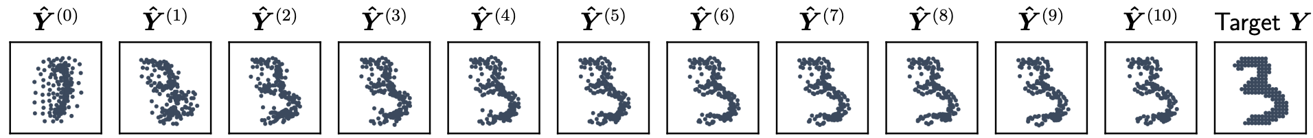
While a cool idea, the gradient iteration learned by DSPN is a flow field (see Fig. 1), and it necessarily requires many iterations to reach the final prediction. Instead, we can learn a permutation-equivariant operator that directly outputs the required set.

Attention is All You Need, Really

Not too long ago, Vaswani et al. showed that we could replace RNNs with attention, causal masking, and position embeddings. It turns out that discarding causal masking and position embeddings leads to self-attention that is permutation-equivariant, as explored in Lee et al., “Set Transformer”, ICML 2019. If this is the case, can we build a model similar to DSPN, but with a transformer instead of the inner gradient-descent inner loop? Of course, we can! There are several advantages:

• The initial set can be higher-dimensional (in DSPN, it has to be the same dimensionality as the output set), leading to more degrees of freedom.
• Transformer layers can operate on the set of different dimensionality, and they do not have to project it to the output dimensionality between layers. This might seem trivial, but it relaxes the flow-field constraint, and in practice, creates transformations that can hold on to some additional state, akin to RNNs.
• DSPN captures dependencies between individual points only via a pooling operation in its DeepSet encoder. Transformers are all about relational reasoning, and can directly use interdependencies between points to generate the final set.

We explored this idea in two recent papers; both published at the ICML 2020 Object-Oriented Learning workshop,

• Kosiorek, Kim, and Rezende, “Conditional Set Generation with Transformers”, where we introduce the Transformer Set Prediction Network (TSPN). TSPN uses an MLP to predict the required number of points from a conditioning, samples the required number of points from a base distribution, and transforms them using a Transformer, see Fig. 2 for an overview.
• Stelzner, Kersting, and Kosiorek, “Generative Adversarial Set Transformers” introduces GAST: a similar idea, where a number of points from a base distribution are conditionally-transformed (based on a global noise vector) using a Transormer. We then use a Set Transformer to discriminate between the generated and real sets.

The same idea was concurrently explored by at least two other groups¹². While details differ, the main finding is that an initial set (randomly-sampled or deterministic and learned) passed through several layers of attention leads to state-of-the-art set generation. The general architecture is as follows:

• Some (big) neural net encoder for processing the conditioning, e.g., a ResNet for images.
• The encoder produces some key-and-value vectors.
• We take either a deterministic or randomly-sampled set of queries and attend over the key-and-value pairs.
• The result might be post-processed by self-attention and/or point-wise MLPs.
• We apply a permutation-invariant loss function, one of the described above. Hungarian matching seems to give the best results.

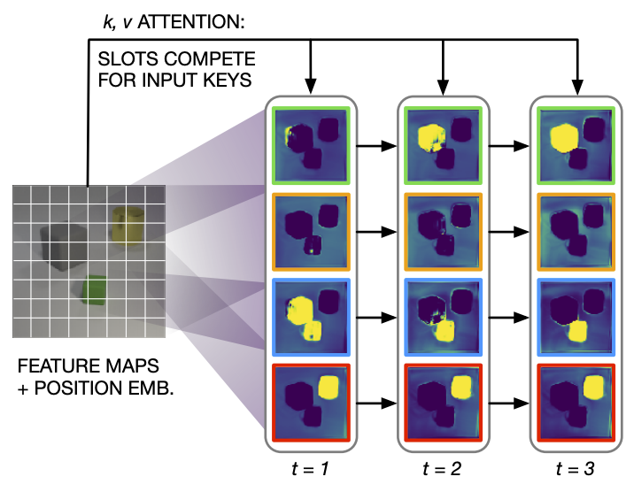
The results of Carion et al.’s DETR model are particularly impressive. While it still required quite a bit of engineering, this pure set-prediction approach achieves state-of-the-art on large-scale object detection on COCO! Locatello et al. show that the particular form of attention required might depend on the task; in their experiments, they normalize attention across the query axis (instead of the key axis), which leads to competition between queries, and provides superior results for unsupervised object segmentation (Fig. 3).

What about those Point Processes??!!

While the above approaches definitely work for generating sets, they make no use of the well-known area of statistics concerned with modeling sets: point processes! Point processes treat the set size \(k \in \mathbb{N}_+\) as a random variable and model it jointly with the set membership \(X \in \mathcal{X}^k\), thus modeling the joint density \(p(X, k)\). This is in contrast to some of the previously-described methods; e.g., DSPN uses heuristics to determine the set size, which does or does not work depending on which loss function it is used with (see our TSPN paper for details). Our TSPN is not much better in that regard, and casts determining the set size as a classification problem–this works quite well in practice, but it cannot generalize to set sizes not seen in training. While a detailed description of point process would take too much space to fit in this blog, I would like to highlight one notion, which I learned about from an excellent paper by Vu et al. called “Model-Based Multiple Instance Learning”.

Let \(f_k(X) = f_k(x_1, ..., x_i, ..., x_k)\) be a probability density function defined over sets of \(k\) elements, and let this density be invariant to ordering of the elements of the set, that is \(\forall \pi\): \(f(X) = f(\pi X)\). It turns out that we can use this density to compare sets of the same cardinality with each other in terms of how probable they are (i.e., how high their likelihood is), but, even if we have two such functions for sets of cardinality \(k\) and \(m\), we simply cannot use them to compare sets of those different cardinalities. Why is that? Well, comparing sets of two and sets of three elements is a bit like comparing square meters m\(^2\) and cubic meters m\(^3\), or like comparing apples and oranges. It is not that we cannot compare sets of different cardinality, but we have to first bring them into the same space, which in this case is dimension-less. To do that, we have to account for a) the number of possible permutations of each set, and b) the unit volume (in case of metric space and comparing m\(^2\) and m\(^3\), we need to figure out how big a meter m\(^1\) is). This leads to the following definition of the probability density function of a set of size \(k\),

where \(p_c(k)\) is the probability mass function of the set size, \(k!\) accounts for all possible permutations of set elements \(\mathbf{x}_i\), \(U \in \mathbb{R}_+\) is the unit volume expressed as a scalar value, and \(f_k\) is the permutation-invariant density of a set of size k. Interestingly, none of the above set-generation papers take the point-process theory into account when defining their likelihoods over sets. I would be curious to see if it improves results, as Vu et al. suggest.

Set To Set

Given the knowledge of how to solve set-to-vector and vector-to-set problems, it should be quite clear how to solve a set-to-set problem: we can encode a set into a vector, and then decode that vector into a set using one of the above vector-to-set methods. While correct, this approach forces us to use a bottleneck in the shape of a single vector. Perhaps a better option is to encode a set to an intermediate set, possibly of smaller cardinality, and use that smaller set as conditioning when generating the output set. There are many methods of how this can be done, and I will only mention that we explored some such problems in Lee et al., “Set Transformer”, ICML 2019 and encourage curious readers to look at the paper.

Outlook and Conclusion

Thank you for reaching this far! We have covered some basics of set-oriented machine learning by taking a look at set-to-vector, vector-to-set, and set-to-set problems and some approaches to solving them. I find this area of ML incredibly interesting, for the variety of things that we consider in life as sets is endless. At the same time, the set-learning models tend to be both theoretically- and architecturally- interesting. Moving forward, I would like to see more models directly based on the point-process theory. Another area that I have not mentioned, and one that is extremely applicable, is that of normalizing flows. You can read about the basics of normalizing flows in my previous blog post, but in short, they are used to transform a simple probability distribution into a more complicated one. As such, there is nothing preventing us from using flows to transform a distribution over independent variables into a joint distribution over sets. While there are some papers that use this idea¹³ to define permutation-invariant likelihoods, none of them uses point-process theory. I will leave working out how to combine flows and point processes as an exercise to the reader, and I will be looking out for papers doing that :)

Further Reading

If you want to learn about point processes, I would recommend:

• The excellent and yet a very short book “Poisson Process” by J. F. C. Kingman.
• The open MIT course on Discrete Stochastic Processes by Robert Gallager, which provides a very gentle introduction to point processes without any measure theory.

Footnotes

Acknowledgements

I would like to give huge thanks to Fabian Fuchs, Thomas Kipf, Hyunjik Kim, Yan Zhang, George Papamakarios, and Danilo Rezende for insightful and inspiring discussions about the machine learning of sets. I would also like to thank Hyunjik Kim and Fabian Fuchs for their feedback on the initial version of this post. This post would not happen if not for Juho Lee, who got me interested in sets in the first place.